Harmonic Functions: Why They’re Nifty

Harmonic functions arise in countless engineering and physics applications. This post will review the definition, associated properties and typical applications of these mathematical marvels.

The Problem

In one dimension, Laplace’s Equation is the differential equation $u^{\prime\prime}(x) = 0$, where $u(x)$ is a twice-differentiable scalar function defined on some open subset of the real number line, i.e., $u(x): \, \Omega \subset  \mathbb{R}$  $\to \mathbb{R}$. The only non-trivial solutions are constant functions like $u(x) = \pi$ or linear functions like $u(x) = 2x + \pi$.

A note on notation: twice-differentiable functions are denoted $C^2$. For more detail, see this Wiki.

More generally, if $u(x)$ is $C^2$ and $u(x) :\, \Omega \subset  \mathbb{R}^{n}$  $\to \mathbb{R}$, $x=(x_1, x_2, … , x_n)$, Laplace’s equation is the homogeneous linear partial differential equation:

$$\begin{eqnarray}
\Delta u(x) ={\partial^2 u \over \partial x_1^2}  + {\partial^2 u \over \partial x_2^2} + … + {\partial^2 u \over \partial x_n^2}= \sum_1^n {\partial^2 u \over \partial x_i^2} = 0
\end{eqnarray}$$

The left-hand side symbol above, $\Delta u(x)$, is called the Laplacian and is sometimes denoted $\nabla^2$ instead which is also just $ \nabla \cdot \nabla u$.

The solutions of $\Delta u(x) = 0$ are called harmonic functions. The name has its root in the study of harmonic motion (sound waves, for example) but the equation has proven applicable to a whole universe of problems beyond that. As will be shown, harmonic functions only become interesting in the context of specific boundary conditions and singularities.

Note: Laplace’s equation can also map complex values, $u(x) :\, \Omega \subset  \mathbb{C}^{n}$  $\to \mathbb{C}$

Properties and Examples

It’s helpful to provide a few examples first. Namely what kind of functions are harmonic? Constant and linear functions certainly fit the bill since their second derivatives are always zero. The rest are, of course, non-linear. For example,

$e^x siny + x + 1$
$x^2 – y^2 + x$
$e^{-x}\, (x\,siny \,-\, y\,cosy)$

They can be complex-valued as well:

$f(z) = (x + iy)^2 = x^2 -y^2 + 2xyi$

Harmonic functions are linearly superimposable, which means that sums and scalar multiples of harmonic functions are themselves harmonic. So based on the examples above we can conclude that $e^x siny + x + 1  + 4(x^2 – y^2 + x)$ is also harmonic. And so on.

Harmonic functions are also invariant under rigid motions, meaning harmonic functions can be translated and rotated and still retain their harmonicity. For examples of this, see this Wiki page.

On their own these two properties, invariance and linearity, are incredibly powerful and yet it’s only the tip of the iceberg…

The Mean Value Property

The mean value property (MVP) is arguably its most important property as it describes how a harmonic function behaves within bounded regions. The outcome may seem strange, but inside any bounded spherical region, the average value of a harmonic function will be its value at that sphere’s center. Stranger still, this is also the average value found on the surface of that sphere. This is true in n-dimensions too, from a line to a circle to an n-sphere.

The mean value property can be expressed mathematically as shown below.

$$\begin{eqnarray}
\def\avint{\mathop{\,\rlap{-}\!\!\int}\nolimits}
u(x_0)
= \avint_{ B(x_0,r)} u dy
= \avint_{\partial B(x_0x,r)}u dS
\end{eqnarray}$$

Some of the symbols here may be unfamiliar. $B(x_0,r)$ is shorthand for an n-dimensional sphere of radius $r$ centered at $x_0$. The symbol $\partial B(x,r)$ refers to the boundary of that sphere (the skin of an apple, if you will). Lastly, the dashed integral symbol is shorthand for the average value of the function inside the region, divided by the volume of that region:

$$\begin{eqnarray}
\avint_{ B(x_0,r)} u dy = {1 \over Vol} \int_{ B(x_0,r)} u dy
\end{eqnarray}$$

In the case of a surface integral, integrate over the surface and divide by the surface area instead.

$$\begin{eqnarray}
\avint_{ \partial B(x_0,r)} u dS = {1 \over Area} \int_{ \partial B(x_0,r)} u dS
\end{eqnarray}$$

Hence, the MVP equation asserts that these two averages are both equal to value of the function at the sphere’s center. Pretty cool, eh? The proof for the MVP is widely available [EV] (§2.2.2) [AXL] [SG].

Two consequences of this. First, extrema can only occur on the boundary: there are no max or min within the region unless the function is constant. And related, if a harmonic function is bounded on all of  $\mathbb{R}^n$ it is necessarily constant.

In his 1881 Treatise on Electricity and Magnetism, James Clark Maxwell made the following remark about the Laplacian:

I propose therefore to call $\nabla^2q$ the concentration of q at the point P, because it indicates the excess of the value of q at that point over its mean value in the neighbourhood of the point.

That is, the Laplacian at a point measures how much a function differs from its neighbors. If it’s positive, then it’s less than its neighbors; if it’s negative, it’s greater. And when it’s zero, this value is exactly the average of those neighboring points [LRX]. This has an interesting application in the problem of edge detection in digital images—sudden changes in the color intensity that occur where the content changes: a face against a background. For this reason, the Laplacian is often used to detect these types of intensity changes [AIS].

Real Analytic and Complex Analysis

Harmonic functions are real-analytic. Being real-analytic on an open set means that the value of the function at any point in that set can be expressed as a convergent power series. As it turns out, that power series is a Taylor series. As a consequence, harmonic functions are also infinitely differentiable, a.k.a., smooth or regular.

Note: The reverse is not true: a smooth function isn’t necessarily analytic. See this example.

In two dimension, harmonic functions have a symbiotic relationship with complex analysis. This leads to a number of interesting outcomes.

The first is that two dimensional harmonic functions are also analytic (holomorphic) and vice versa. Analytic is the complex version of differentiable, which is more powerful since it requires the derivative at a point be the same from every direction, not just right and left as it is with real differentiability.

Next, if a function is analytic, then its real and complex parts are harmonic. This follows from the Cauchy-Riemann equations.

Dirichlet Problem

When the Laplacian yields something other than zero, the resulting inhomogeneous equation is called Poisson’s equation, $\Delta u(x) = -f(x)$. It should be noted that a solution to Poisson’s equation can be linearly combined with a harmonic function and still be a solution.  More on Poisson’s equation shortly.

The problem of solving a PDE with a specific boundary function is called the Dirichlet problem. The solution of the Dirichlet problem for the Laplace equation, and thus for a harmonic function, if it exists, will be unique. As a consequence, the solution inside the region is uniquely defined by it values on the boundary.

$$\begin{eqnarray}
\begin{cases}
\phantom{-}
\mathop{{}\bigtriangleup}\nolimits
u = 0 \,\,u \in \Omega
\\\phantom{-}
u(x) = g(x) \,\,\,\,u \in \partial \Omega
\end{cases}
\end{eqnarray}$$

This is an example of a well-posed problem, which basically means that its solutions represent something realistic and are not pathological. In particular, solutions will continuously approach the boundary function value as $x$ nears the boundary $\partial \Omega$ (this is the notation for the boundary of $\Omega$).

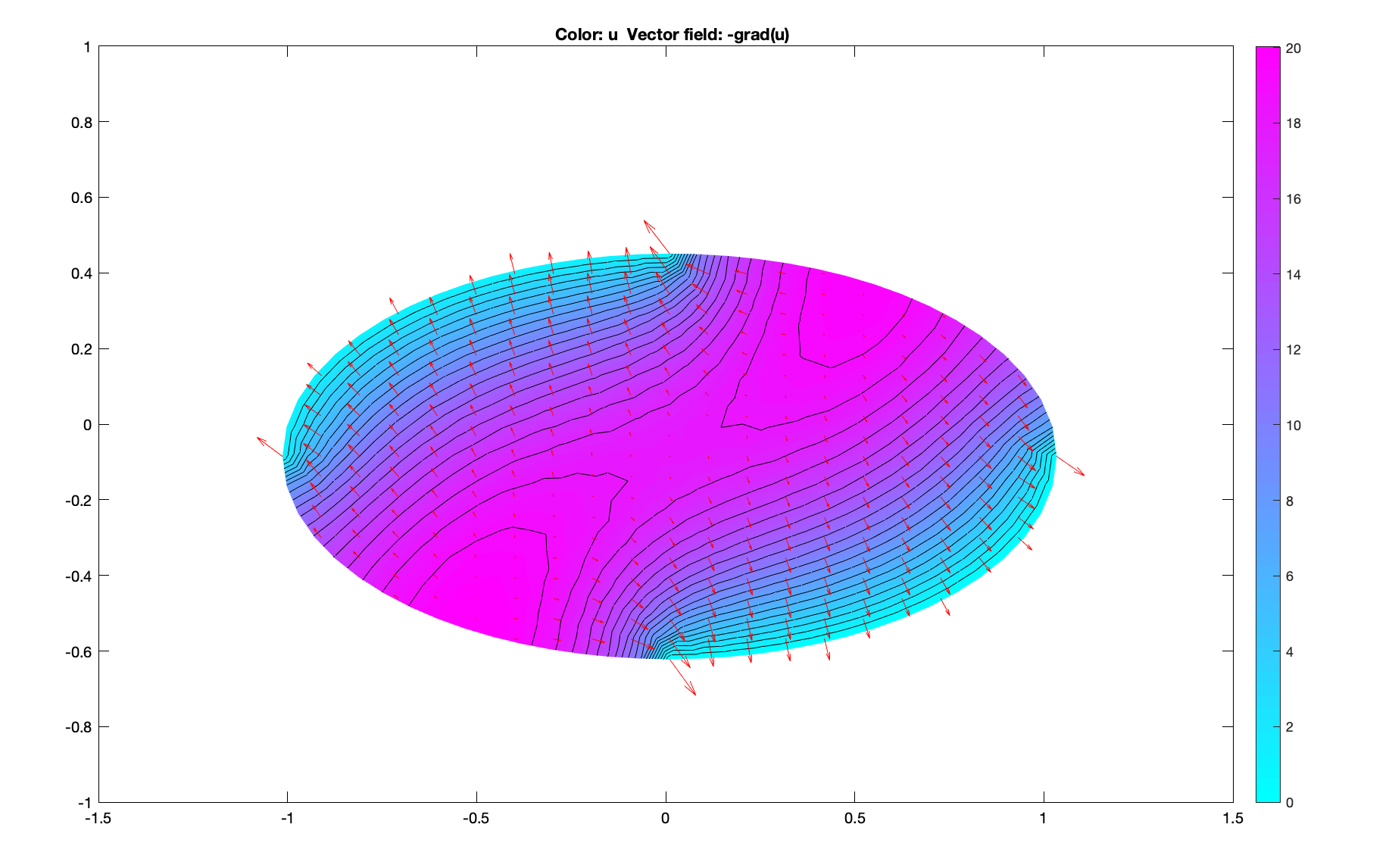
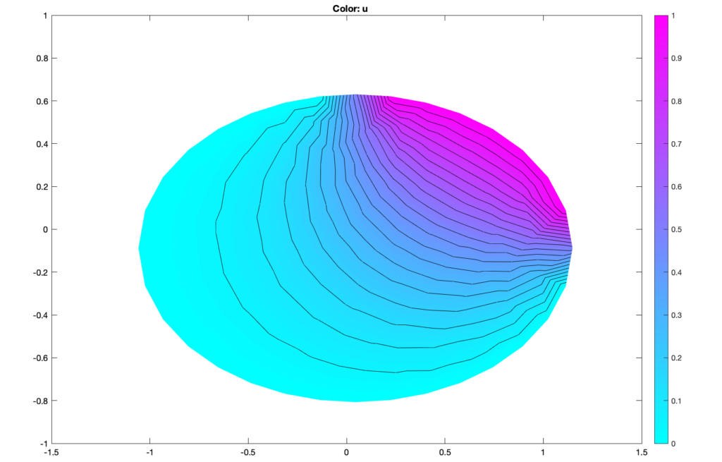
The canonical example of a Laplace Dirichlet problem is a steady-state temperature distribution in a region with one or more heated edges. The image below is an example of this (via Matlab). There are also interesting applications in Brownian Motion.

There are other types of boundary problems too, such as Neumann and Robin depending on how the boundary constraints are defined. For steady-state heat problems, Neumann conditions are often used to represent adiabatic (insulated) edges.

Operators

The notion of a linear operator $L$ is useful when working with these equations. A linear operator is simply a mapping from one vector space to another. In the realm of differential equations, these vector spaces are typically infinite dimensional vector spaces of real or complex-valued functions subject to constraints.

For example, the space of real-valued continuous functions on an open set or the space of twice-differentiable complex functions over the real numbers. $L^2$ is one that often arises in Quantum Mechanics. In all cases, the vectors in these vector spaces are functions. These vector spaces can also be endowed with a norm, which provides a notion of length, and an inner product, which provides a notion of angles, the canonical of which is a Hilbert Space.

The linear part of “linear operator” means that the operation on a sum of terms is the sum of those operations: $L(\alpha x + \beta y) = \alpha L(x) + \beta L(y)$. For harmonic functions, this is consistent with the property of linear superposition already mentioned.

Familiar calculus expressions like the derivative can be expressed as linear operators, for example, $L=\frac{d}{dx}$ or in terms of the function on which it operates, $L(u) = u^{\prime}$.

This is an example of a linear differentiable operator, one that maps a differentiable function $u(x)$ to a linear algebraic expression of derivatives. For example, $L(u) = u^{\prime\prime} + 2u^{\prime} + u$. Relevant to this discussion, the Laplacian is the linear differential operator, $ L= \Delta $.

There are many vector spaces on which these differential operators can “operate.” The vector space of twice-differential functions, $C^2(\mathbb{R})$, for example. Or the space of infinitely differentiable (or smooth) functions $C^{\infty}(\mathbb{R})$ and so on. The point being that a linear operator must have both a linear operation (e.g., the derivative) and a vector space on which it operates.

There are many other types of linear operators. In a system of linear equations, the matrix can be treated as an operator as can its inverse. And on the topic of inverses, the inverse operator for the first derivative operator is the antiderivative.

Operators have null spaces (sometimes called the kernel, which is a poor naming choice since the kernel has an unrelated meaning as will be shown below). These are the functions that the operator maps to zero: $Lu=0$, i.e., $\Delta u =0$. In particular, harmonic functions are the null space of the Laplacian operator.

In operator form, Poisson’s equation takes on the following elegance.

$ L = \Delta$ (the operator)
$ L u = f $ (Poisson’s equation)
$ u = L^{-1}f $ (its solution!)

With this in mind, the inverse of this operator is the following integral equation

$$\begin{eqnarray}
u = L^{-1}f  =\int_{\Omega} G \, f \, d{\Omega}
\end{eqnarray}$$

The new term $G$ is called the kernel of the integral operator. For a linear differential operator, this is just the Green’s functions, discussed below. Thus knowing the kernel one can (theoretically, at least) construct a general solution to the differential equation.

Now you may be staring at this thinking, “what if $f = 0$?” as it does with harmonic functions. As written above, this would mean that $u$ is always the zero function, which would make this a very dull topic. The reason this is wrong is because we omitted the boundary conditions, which (as you probably know) are required when solving a differential equation. The operator therefore must also account for those and in doing so, the integral equation will have to include additional terms to represent the boundary conditions. Note that with these types of operators, the boundary conditions are actually embedded into their definition.

The boundary of $\Omega$ is denoted $\partial\Omega$ and so the revised solution will be of this form:

$$\begin{eqnarray}
u = L^{-1}f  = BC(\partial\Omega) +\,\, + \int_{\Omega} G \, f \, d{\Omega}
\end{eqnarray}$$

This is demonstrated below in the discussion of Poisson Dirichlet problems.

Finally, note that just as it is with matrices, this inverse, and thus the solutions we seek, only exists if there are no non-trivial solutions in the null space. In matrix language, this means that all the eigenvalues are non-zero. The same holds with operators: the $ \lambda$ of $ L u = \lambda u $ are non-zero too.

The Fundamental Solution

The fundamental solution of Laplace’s equation is a function $\Phi(x| \xi)$, which is harmonic everywhere except at a singularity $\xi$. As an operator this is often written $L \Phi(x| \xi)= \delta(\xi)$, where $\delta(\xi)$ is a Dirac distribution centered at $\xi$. A classic example is the potential field generated by a unit point charge.

There are three types of fundamental solution for Laplace’s equation, depending on the dimensionality of the problem.

• If $n=1$ the fundamental solution is a linear function $|x – a|$
• For $n=2$ it’s logarithmic: $ln |x – a| \,, x \ne a$
• For $n \ge 3$ it’s $|x – a|^{2-n}  \,, x \ne a$

A few observations around this. The first is that these represent a family of solutions, not a specific one. This is because one can add harmonic functions to this solution without changing the outcome.

The second observation is that for $n>1$, the solutions above are not defined at the the point $a$, rather, they are only harmonic on the so-called “punctured region,” $\Omega \backslash \{a\}$. But none have a derivative at $a$. The singularity that occurs there is of tremendous importance.

Third, these equations have radial symmetry. This again aligns with intuition. Both heat and electric fields radiate radially outward, as does the pull of gravity.

Free space Poisson equation

The Poisson equation can be expressed in terms of the fundamental solution, the so-called free space solution. Again, in the absence of boundary conditions, non-trivial solutions arise as the result of a singularity. This is captured by the Dirac distribution. We can start by using a property of the Dirac distribution called the “sifting property” where $\xi$ represents the point where the singularity occurs.

$$\begin{eqnarray}
\int_{\mathbb{R}^n}\delta (x-\xi) \, f(x)dx
=
f(\xi)
\end{eqnarray}$$

We can shorten this by writing it as a convolution.

$$\begin{eqnarray}
\delta (x – \xi) * f(x)
=\int_{\mathbb{R}^n}\delta (x-\xi) \, f(x)dx = f(\xi)
\end{eqnarray}$$

Convolutions have a useful property with respect to differentiation, shown here in the one-dimensional case but true in general too.

$$\begin{eqnarray}
\frac{d}{dx} (f(x) * g(x))
=\frac{df}{dx}  * g(x) =f(x) * \frac{dg}{dx}
\end{eqnarray}$$

It also has a commutative property that allows swapping the order of the convolution

$$\begin{eqnarray}
f(x) * g(x)
=\int_{\mathbb{R}^n}f(x-\xi) \, g(x)d\xi
=\int_{\mathbb{R}^n}f(\xi) \, g(x- \xi)d\xi
\end{eqnarray}$$

Putting these together

$\mathop{{}\bigtriangleup}\nolimits \Phi (x | \xi) = \delta(\xi)
\implies$

$\mathop{{}\bigtriangleup}\nolimits( \Phi (x | \xi) * f(x) ) =\mathop{{}\bigtriangleup}\nolimits( \Phi (x | \xi) ) * f(x)  =$

$\delta(x – \xi)  * f(x)
= \delta(\xi)  * f(x – \xi) = f(x)$

This means that we can express the solution to the free space Poisson equation as a convolution of the fundamental solution with the driving function, $f$.

$$\begin{eqnarray}
u(x) =\Phi(x| \xi) * f(x) =\int_{\mathbb{R}^n}\Phi(x| \xi) \, f(\xi)d\xi
\end{eqnarray}$$

One caveat: the function $f$ must only be non-zero inside a finite sphere, or in mathematical terms, it must have compact support. Compact support on a closed interval $[a,b]$ is denoted with a zero subscript, as in $C_0[a,b]$.

Green’s Functions

Heads up, we do a deep-dive of Green’s functions in this post. Check it out.

The Green’s function $G(x, \xi)$ for Poisson’s equation is a fundamental solution with homogeneous boundary conditions applied. It is sometimes called the Influence function. As mentioned above, these represent the kernel of the inverse differential operator, $ u = L^{-1}f $.

The second variable in $G(x, \xi)$, $\xi$, indicates that we define a Green’s function at every point in the region thus providing a mechanism to superimpose them across that region. We set $G(x, \xi)$ to zero on the boundary so that the only component of $u(x)$ on the boundary is $g(x)$, the boundary value function. Green, in his seminal 1828 paper in which this concept was introduced, suggested that we think of the zero potential on the boundary as the result of grounding the conducting surface. But this technique proved to extend far beyond problems in electrostatics.

Collectively, these ideas are expressed by the following accessory equation:

$$\begin{eqnarray}
\begin{cases}
\phantom{-}
\mathop{{}\bigtriangleup}\nolimits
G(x, \xi) = \delta(x – \xi) & u \in \Omega
\\\phantom{-}
G(x, \xi) = 0 & u \in \partial \Omega
\end{cases}
\end{eqnarray}$$

Green’s functions are specific to the boundary geometry too, meaning they can be reused when solving the Dirichlet Problem for the same region regardless of the forcing and boundary functions.

One side note. The Green’s function here is symmetric (or more formally, self-adjoint). That is, $G(x, \xi) = G(\xi, x)$. The proof of this is complicated (see [EV]) but the upshot is that we can switch variables when doing certain integrations. This comes in handy when proving some of the results shown in this section.

It’s also worth stressing that Green’s functions exist for many different differential equations, not just Poisson’s equation. It is but one of the many techniques available for cracking these often intractable problems. We now demonstrate how it is used in the context of the Dirichlet Problem.

Poisson Dirichlet Problem 

In terms of the Green’s function, the general solution for the the Poisson equation with Dirichlet conditions is shown below. The proof is shown in [EV], [SG] and others. But it should look familiar based on the discussion of inverse differential operators above.

$$\begin{eqnarray}
u(x) =
– \int_{\partial \Omega} g(\xi)\frac {\partial G(x, \xi)}{\partial \eta} dS(\xi)
+ \int_{\Omega} f(\xi) G(x, \xi) d\xi
\end{eqnarray}$$

The term $\frac {\partial G(x, \xi)}{\partial \eta} $ is called the Boundary Influence Function, which for the two dimensional circle of radius $R$ becomes the well-known Poisson Kernel. Note that this is just the derivative of the kernel of the inverse operator with respect to the unit normal of the boundary.

In particular, when $f(x)=0$ as it is for Laplace’s equation, the second term vanishes leaving the following closed-form solution:

$$\begin{eqnarray}
u(r, \theta) = \frac{1}{2\pi R}\int_0^{2\pi}
\frac
{R^2 – r^2}
{ r^2 – 2Rr\cos(\theta – \psi) + R^2} g(\psi)
d\psi
\end{eqnarray}$$

You should notice that the denominator above has a singularity at the point $(R, \psi)$. The Poisson Kernel therefore represents the value that would be generated by a delta distribution on the boundary per the singularity in the denominator. This means that the function value $u(r, \theta)$ is the weighted sum of all such distributions along the boundary. Compare this to how the forcing function is the weighted sum of Green’s functions across that region.

The Poisson Kernel for the unit circle can be expressed in rectangular coordinates using the law of cosines:

$$\begin{eqnarray}
u(x) =
{1 -|x|^2 \over 2 \pi}
\int_{\partial \Omega} \frac {g(\xi)}{|x-\xi |^2} d\xi
\end{eqnarray}$$

More generally in n-dimensions,

$$\begin{eqnarray}
u(x) =
{1 -|x|^2 \over n \alpha(n)}
\int_{\partial \Omega} \frac {g(\xi)}{|x-\xi |^n} d\xi
\end{eqnarray}$$

In general, finding the Green’s functions and thus solving Poisson’s equation is not easy since these integrals generally do not have closed-form solutions. But solutions do exist for a few simple geometries (i.e., the shape of the boundary). The solution on a circle is well-known as is the solution in the half-plane both found using the method of images (see [EV], for example).

Fortunately in two dimensions there are many more options thanks to correspondence between harmonic functions and complex analysis. In particular, we have the wonderful technique of conformal mappings and by extension, the technique of Schwartz-Christoffel. For example, this is the two-dimensional unit circle Green’s function translated from another region via a conformal mapping $g(z)$:

$$\begin{eqnarray}
G(z, \xi) =
{1 \over 2\pi} \ln{
|{1 – \overline g(\xi) g(z) } | \over {|g(z)-g(\xi)|}
}
\end{eqnarray}$$

Exterior Problems

Exterior solutions are also interesting. In two dimensions, the exterior solution to the Dirichlet problem on a disc tends toward a finite limit that happens to be the mean value solution. That is, the solution at infinity for an exterior region of a disc is that same as the value at the center of the disc interior. This can be shown fairly easily by taking the limit toward infinity of the Poisson Kernel in the exterior Dirichlet Problem.

$$\begin{eqnarray}
\lim_{r\to\infty}
u(r, \theta) = \frac{1}{2\pi }\int_0^{2\pi}
g(\psi)
d\psi
\end{eqnarray}$$

In higher dimensions, this limit needs to be zero to ensure a unique solution. For a proof see [AXL] or this paper by Giles Auchmuty and Qi Han. This result is interesting given the previous result for the two-dimensional problem and arguably physically consistent too. See [SG].

Bibliography

[AIS] Sinha, U. The Sobel and Laplacian Edge Detectors. Microsoft.

[ALF] Ahflors, L., 1979, Complex Analysis, McGraw-Hill Book Company.

[AXL] Axler, S., Bourdon, P., Ramsey, W., 2001, Harmonic Function Theory, Springer.

[EV] Evans, L., 2010, Partial Differential Equations: Second Edition (Graduate Studies in Mathematics), 2nd Edition,American Mathematical Society.

[EV2] Evans, L. 2011?. Overview article on partial differential equations, UC Berkeley.

[HT] Hunter, J., 2001. Applied Analysis, WSPC.

[HT2] Hunter, J., 2014. Notes on Partial Differential Equations, University of California at Davis.

[LRX] Lamoureux, M., 2004. The mathematics of PDEs and the wave equation. Univ. of Calgary.

[LV] Levandosky, J., 2003. Math 220B Lectures, Stanford University.

[NH] Nehari, Z., 1952, Conformal Mapping, McGraw-Hill Book Company.

[OL2] Olver, P., 2018, Complex Analysis and Conformal Mapping, University of Michigan

[STR] Strauss, W. 2007. Partial Differential Equations: An Introduction, Wiley.

[SG] Stakgold, I., 1967,Boundary Value Problems of Mathematical Physics, Macmillan.